JPEG Compression Implementation

We broke the process of compressing an RGB image into seven main steps that we implemented in MATLAB. In order to decompress the image, the same seven steps need to be reversed, so we wrote the inverse to each of these steps as well. Here are seven steps to compress an image:

1. Resize The Image

We wanted our program to be robust enough to take in any image, but only certain image sizes would work with our algorithm. In order for the compression to work, the height and width of the image needed to be divisible by eight. So in this function, an image is converted to a matrix, and if it’s dimensions are not divisible by 8, then the appropriate amount of rows or columns are added as padding to make the image the correct dimensions. These values are saved for later unpacking.

2. Convert it to the YCbCr color-space

Generally, the color of an image is defined by its RGB - red, green and blue - values from 0 to 255. However, this is not the only way to define the color of a pixel. YCbCr encodes the color in terms of luminance, chrominance red and chrominance blue. YCbCr is used by JPEG compression because of the discovery that our eyes are much more responsive to changes in light than to changes in color. So in order to save more important information it makes sense to save information about the brightness of an image - that way, we can get rid of a lot of color information without creating a noticeable difference in the image.

This function converts an RGB matrix to a YCbCr matrix by iterating over every pixel and transforming it by the appropriate operation, as can be seen in the image above. This turns the three NxN RGB matrices to three NxN YCbCr matrices of values from [0, 255].

3. Shifting The Values to Center Around Zero

This function shifts all the values to a range from -128 to 127 so that the matrix is ready for the blocking step. Additionally, this also creates a signal centered around zero, which is important for the DCT, as all sinusoidal transforms assume the signal is centered around zero.

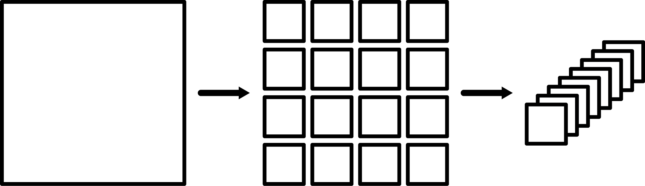
4. Convert into 8x8 Blocks

Next, the image is broken up into 8x8 or smaller chunks and stacked into a list, as shown below.

To understand why this is done, we can think about the number of operations needed to compute the DCT.
A Note on Computational Complexity
In computer science, the computational complexity of a function or algorithm is, in simplest terms, the number of operations needed to compute the function on an input of an arbitrary size. We can look at the computational complexity of the DCT to understand why it’s advantageous to break an image into smaller chunks. The operation of multiplying an NxN image matrix by an NxN DCT matrix requires a number of operation proportional to $N^3$; as a result, it’s advantageous to break the image into smaller chunks and take the DCT of each of the chunks.

5. Take the DCT

At this point, we’re ready to take the DCT of each block. In our implementation of JPEG, we wrote our own implementation of the DCT based a DCT matrix that we compute manually. For more information on how the DCT works, look at our page on the DCT.

6. Quantization

Next, we use quantization to get rid of information in certain frequencies. The objective of quantization is to make as many frequencies the same as possible, usually by driving them to zero. This is accomplished by dividing each DCT chunk by a quantization matrix and rounding values down. A quantization matrix is a matrix that reduces the higher frequencies of the DCT by much more than the lower frequencies - as a result, in most images, many of the high frequencies will become zero, and the lower frequencies will stay as nonzero values.

Recall from earlier that JPEG uses YCbCr color-space because it separates brightness and color components, and brightness changes are more easily seen by the human eye than color. This manifests itself in the quantization matrices: JPEG uses a different quantization matrix for brightness and color, with the color matrix reducing most higher frequencies much more than the brightness matrix.

7. Encoding

The final step is to encode the data. In our implementation, we use Huffman encoding to encode our JPEG data. Huffman coding takes the DCT matrix and converts it into a stream of bits - it takes advantage of repeated elements in the DCT to reduce the number of bits needed to store the encoded data. Note that this is the optimal format in which to store the data, as this is the state in which storing the image data requires the lowest number of bits, since this stream of bits is going to be much smaller than the original image data where ever pixel is 8 bits.

Decoding

In order to retrieve the image data and reconstruct it, we have to decode it. To do that, we do the inverse of every operation, in backwards order. Note that when undoing the quantization, we dequantize by multiplying by the quantization matrix, instead of dividing. However, this is where information actually gets lost in JPEG compression; because of the rounding step in the original quantization, some frequencies have been reduced to 0, and they will stay 0 even after dequantization. Ultimately, we end up with a reconstruction of the original image that has some amount of data lost.